

8 January 2015
We're going to recap the power of the Tableau “self blend” before drilling into potential issues you might face given the structure of your underlying data. As the title of the blog suggests we'll then explore how “data padding” can help resolve those issues.
Introduction
I want to take a moment to recap the power of the Tableau 'self blend' before drilling into potential issues you might face given the structure of your underlying data. As the title of the blog suggests I'll then explain how 'data padding' can help resolve those issues.The self blend technique involves duplicating an existing data source and invoking a blend between that duplicate and the original. Laszlo covered this recently in Double dynamite - or duplicating the data connection.To set the scene for data padding I'm going work through a couple of blending examples below as an illustration, and for this purpose I'm going to use the Superstore Sales data set as the data source.Self Blends
Example 1 - Sales as a % of Department
[tableau server='public.tableausoftware.com' workbook='SelfBlendsandDataPadding' view='Eg1BasicSelfBlend' tabs='no' toolbar='yes' revert='all' refresh='no' linktarget='' width='470px' height='530px'][/tableau]Here I am calculating the Sales per Category as a percentage of the overall Sales for the Department the respective Category belongs to.Its a simple example to introduce the power of the self blend, the key step being to ensure you blend on Department, but not on Category which Tableau would enable by default.Effectively you return a higher level of aggregation from the Secondary (aggregated by Department) than the Primary (aggregated by Department and Category). When they blend together, the higher level aggregation from the Secondary is repeated for each Category.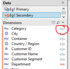
Example 2 - Sales as % of Previous Year
[tableau server='public.tableausoftware.com' workbook='SelfBlendsandDataPadding' view='Eg2PreviousYear' tabs='no' toolbar='yes' revert='all' refresh='no' linktarget='' width='540px' height='400px'][/tableau]Here I'm utilising a calculated field 'Blend Date' in the Secondary for the purpose of offsetting the Order Date by 1 year.DATEADD('year',1, [Order Date] )For consistency I like to have the same named field in the Primary, although it is just defined as a duplicate of Order Date.I'm then asking Tableau to perform a blend on the Year of this date, along with Category. Take care to ensure the blend on the date is operating at the Year.Tip: When blending with dates I like to clear out the automatic relationships and work with custom relationships.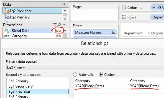
Example 3 - Market Share in Italy
I'm delving a little deeper into the Superstore dataset to setup this example. I've specifically filtered down to a single Country / Region (Italy) with a small subset of active 'States' so we have a concise example. I'm again using a self blend, this time I'm blending on Category, Country / Region and Department. Importantly I have deselected the default blend on State.The crosstab indicates the sum of Sales from the Primary which I am referring to as Market Share, and a sum Sales from the Secondary which I am referring to as Market Value. When you select a State from the map, I am applying a filter action to the crosstab. The desire is to see what share of the Italian market is applicable to each State. Use the viz and observe the results of the filter action:[tableau server='public.tableausoftware.com' workbook='SelfBlendsandDataPadding' view='Eg3MarketShareinItaly' tabs='no' toolbar='yes' revert='all' refresh='no' linktarget='' width='470px' height='720px'][/tableau]The Effect of Sparse Data on Blending
In particular when you select Veneto or Tuscany, you are not seeing the full Italian Market Value. Given what we've seen in the previous examples, we might consider this a little odd. We've taken care to setup the blend correctly, the sum of Sales coming from the Secondary should be agnostic of State. The reason is perhaps subtle, but fundamental to the blending process and order of operations within Tableau. The query over the Primary has aggregated our data by Category and Department, but importantly we have active filters, and both filters and aggregation take place before the blend. The data has been filtered by Country / Region, together with an action filter which is applied on State.To demonstrate, if we revisit the viz above and select Tuscany we will see there are only sales recorded within 5 of the Categories. Hence when blending, we are only considering from the Secondary those Sales which exist in those 5 Categories. The aggregation from the Secondary will still operate over all States, but it cannot include Sales from those other Categories whilst Category is an active blending field.Data Padding
To continue with the Italian example, we have seen how sparse data within one State can impact on our desired output. One solution is to pad out our data by the introduction of extra rows where we have a gap. In this case that would be to ensure Tuscany has rows of data for all other Categories, not just the 5 where actual Sales exist. In general, Tableau does not allow us to inject rows into our data so I'm going to reach into the data connection and demonstrate a technique that is possible with Custom SQL.For this example with Superstore Sales, the mention of Custom SQL comes with a caveat, and that is that I'm going to have to use the Legacy Excel connector to take advantage of JET, and as a result I'm afraid this is going to be PC only. If you're on MAC and have data in Excel you're going to have to do some pre-processing to either get it into a database or utilise a product like Alteryx.To recap the legacy connecter, the trick is to select the appropriate file 'open' option when you locate your Excel file: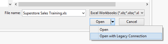 Tip: This one I only discovered a few weeks back. In this instance, drag your sheet into the data window as if you were going to use the visual interface to construct your query. Now use the Data menu option to convert to custom SQL, the field names are pre-populated for you (akin to the default behaviour in v8.1)
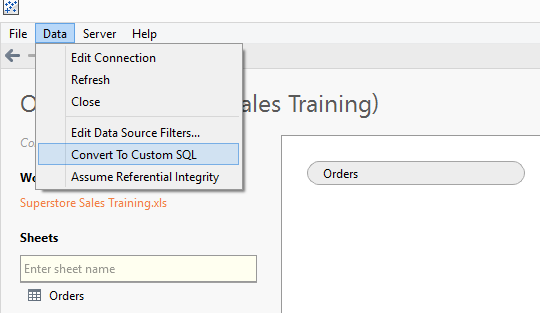 Resulting in:
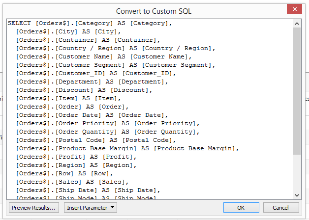 Digression aside, lets move onto the padding technique.... I like to think of this as utilising 2 passes over my data, firstly I will identify all possible combinations that I need for my analysis, and secondly I will enrich this with my actual data.In this case I want to ensure that for each State (within each Country) I have a row for each Category (within each Department).In SQL we might refer to this as the cartesian product of States and Categories. The cartesian product will act as the frame for my data, I can then left outer join the actuals.As I'm using Superstore Sales I have a JET friendly custom SQL statement to achieve this. The cartesian product is the blue section, the join to the actual is orange.SELECT[Cartesian].[State] AS [State],[Cartesian].[Category] AS [Category],[Cartesian].[Department] AS [Department],[Cartesian].[Country / Region] AS [Country / Region],[Full].[City] AS [City],[Full].[Container] AS [Container],[Full].[Customer Name] AS [Customer Name],[Full].[Customer Segment] AS [Customer Segment],[Full].[Customer_ID] AS [Customer_ID],[Full].[Discount] AS [Discount],[Full].[Item] AS [Item],[Full].[Order] AS [Order],[Full].[Order Date] AS [Order Date],[Full].[Order Priority] AS [Order Priority],[Full].[Order Quantity] AS [Order Quantity],[Full].[Postal Code] AS [Postal Code],[Full].[Product Base Margin] AS [Product Base Margin],[Full].[Profit] AS [Profit],[Full].[Region] AS [Region],[Full].[Row] AS [Row],[Full].[Sales] AS [Sales],[Full].[Ship Date] AS [Ship Date],[Full].[Ship Mode] AS [Ship Mode],[Full].[Shipping Cost] AS [Shipping Cost],[Full].[SubRegion] AS [SubRegion],[Full].[Unit Price] AS [Unit Price]FROM
(SELECT [q1].[Country / Region] AS [Country / Region], [q1].[State] AS [State], [q2].[Department] AS [Department], [q2].[Category] AS [Category]FROM
(
SELECT [Country / Region], [State] FROM [Orders$] GROUP BY [Country / Region], [State] ) AS [q1],
( SELECT [Department], [Category] FROM [Orders$] GROUP BY [Department], [Category] ) AS [q2]
) AS [Cartesian]
LEFT OUTER JOIN [Orders$] [Full] ON [Full].[State] = [Cartesian].[State] AND [Full].[Category] = [Cartesian].[Category]