

This post is a complete overview of what market basket analysis is, and how to use the MB Rules and MB Inspect tools to do market basket analysis in Alteryx. If you don't use Alteryx, don't worry - the theory side of things may well still be useful for you!
THEORY
It's Saturday morning in Gwilym's Breakfast Goods Co., and people are slowly rolling in to buy their weekend breakfast ingredients (we don't sell much else). The first five people through the door make the following purchases:
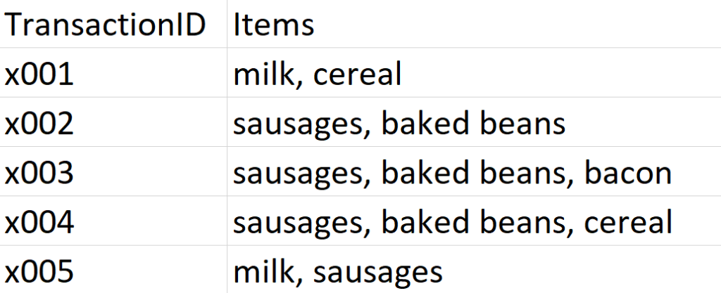
I'm looking at my dataset here, and I can instantly see a couple of insights. Firstly, that's a lot of rich beef sausages we're selling. And secondly, people seem to buy sausages and baked beans together.
This is, in essence, market basket analysis - looking at your transactions to see what people buy a lot of, what people don't buy a lot of, and what different things people buy together. There are four main concepts in market basket analysis - association rules, support, confidence, and lift.
Association rules
An association rule is the name for a relationship between items or combinations of items across all transactions, and it's often written like this:
sausages → baked beans
This means 'if people buy sausages, they also buy baked beans', and we can see that this association rule figures pretty prominently in this dataset. But an association rule is just the name for the relationship, not a statement about the strength of it. For example, milk → sausages is also an association rule, even though there's only one transaction where that happens.
Support
This is just the proportion of transactions that contain a thing. Support can be for individual items (like sausages) or a combination of items (like sausages and baked beans). In our example dataset, the support for sausages is 0.8, because sausages are in four transactions out of a total of five.
Confidence
While support refers to items in the transaction list, confidence depends on association rules. For an association rule, confidence is the number of transactions that contain a thing that already contain the other thing. It's calculated like this:
[support for both items in association rule]
/
[support for item on left hand side of rule]
So, if we use the rule sausages → baked beans , the confidence is 0.75. This is because it's calculated like this:
[support for sausages and baked beans, which is 3 out of 5, or 0.6]
/
[support for sausages, which is 4 out of 5, or 0.8]
If we take the alternative association rule for the same two items, which is baked beans → sausages, then the confidence is 1, because the support for beans and sausages is 0.6, and the support for beans alone is also 0.6.
Lift
Finally, lift is how likely two or more things are to be bought together compared to being bought independently. It's calculated like this:
[support for both items]
/
[support for one item] * [support for the other item]
Unlike confidence, where the value will change depending on which way round the rule between two items is, the direction of a rule makes no difference to the lift value.
Again, if we use the rule sausages → baked beans , the lift is 1.25. This is because it's calculated like this:
[support for sausages and beans, which is 0.6]
/
[support for sausages, which is 0.8] * [support for beans, which is 0.6]
That gives us 0.6 / (0.8 * 0.6), which is 0.6 / 0.48, which is 1.25
A rough guide to lift is that if it's above 1, then it means that the two items are bought more frequently as a pair than they are bought individually, while if it's below 1, then it means that the two items are bought more frequently individually than as a pair.
ALTERYX EXAMPLES
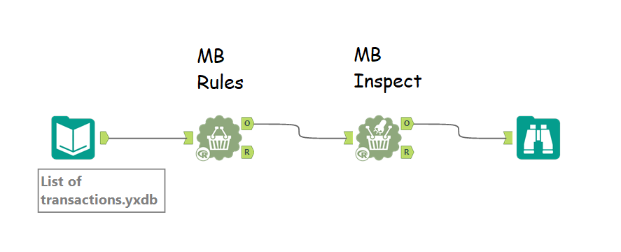
That's pretty much it for the theory so far, so let's create a simple analysis in Alteryx. You'll need two tools - MB Rules and MB Inspect.
MB Rules does all the work, and it's where you set your support and confidence thresholds. However, it only outputs an R object, which Alteryx can't read as a standard data frame... so you need MB Inspect, which is basically a glorified filter tool, to turn that into Alteryx data.
You can set it up a little like this:
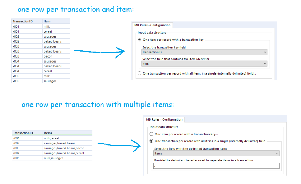
You'll also want to sort out your data beforehand. There are two possible ways you can structure your data for the MB Rules tool to work. You can either have a row for every single item of every single transaction, or you can have a row for every transaction, with each item separated by the same character. The MB Rules tool can handle both structures, and you'd set it up as follows:
Apriori Association Rules
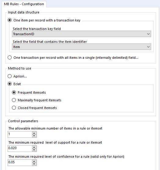
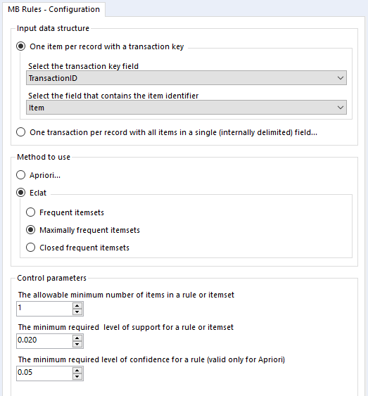
In the MB Rules tool, let's set it up to give us the association rules, with their support, confidence, and lift. You can do that by selecting Apriori and Association rules under method to use:
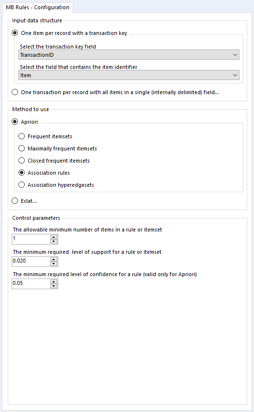
Here, I've left the control parameters to their defaults - 0.02 support for an item or set of items or association rule, and 0.05 for the confidence of an association rule. With the support filter, note that this will apply to both items and association rules. For example, in the five transaction dataset, the support for milk is 0.4 and the support for cereal is 0.4. If I set my minimum support to 0.4, then the empty LHS rules for milk and cereal will come through (more on that in a moment), but the association rule for milk → cereal will not be returned, because the support for that association rule is only 0.2, because both milk and cereal only occur together in one transaction out of five.
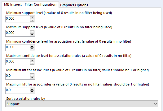
Onto the MB Inspect tool, and I normally leave it like this - zeroes for everything, because I've set most of my filters that I care about in the MB Rules tool.
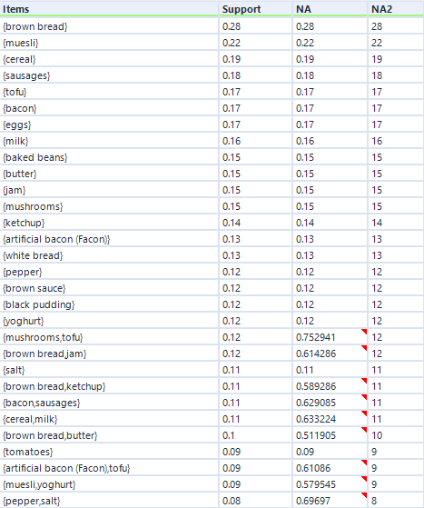
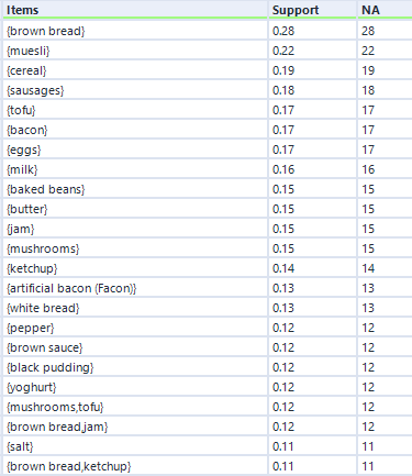
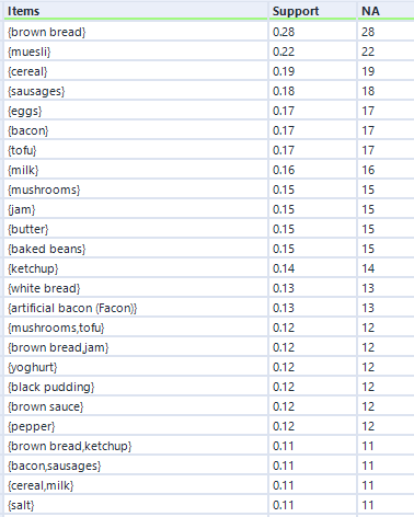
That's pretty much it, so I'll now press run. For this data, I've expanded my dataset from the first five transactions to a hundred transactions. Here are the association rules in my dataset:
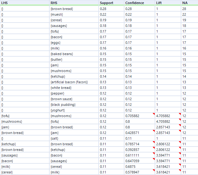
Remember I mentioned empty rules earlier? The top handful of rows where the LHS column is '{}' is what I mean. What this shows is the association rule, if you can really call it that, for items individually, totally independent of other items. This just shows the support for an individual item, and because it's independent of other items, the confidence is the same, and the lift is always 1.
Do you see the NA column on the far right? This is another useful output, although it's not labelled very well. This stands for Number of Associations (I think) - in any case, it's a count of how many transactions this item or set of items occurs in. So, brown bread turns up in 28 transactions out of 100 (hence the 0.28 support for brown bread), and cereal and milk turn up in 11 transactions out of 100 (hence the 0.11 support for cereal → milk).
You can also see how lift is independent of the association rule direction, but confidence isn't. For example, take the two association rules between tofu and mushrooms. The first one, tofu → mushrooms, has a confidence of 0.705882, which means that mushrooms turn up in 70% of transactions that have tofu in them. The second one, mushrooms → tofu, has a confidence of 0.8, which means that tofu turns up in 80% of transactions that have mushrooms in them. Or in other words, 80% of people who buy mushrooms also have tofu, and 70% of people who buy tofu also buy mushrooms. Either way, there's a big lift of 4.7, which means that tofu and mushrooms occur together about 4.7 times more often than you'd expect if 15 people threw mushrooms into their trolley at random and 17 people threw tofu into their trolley at random.
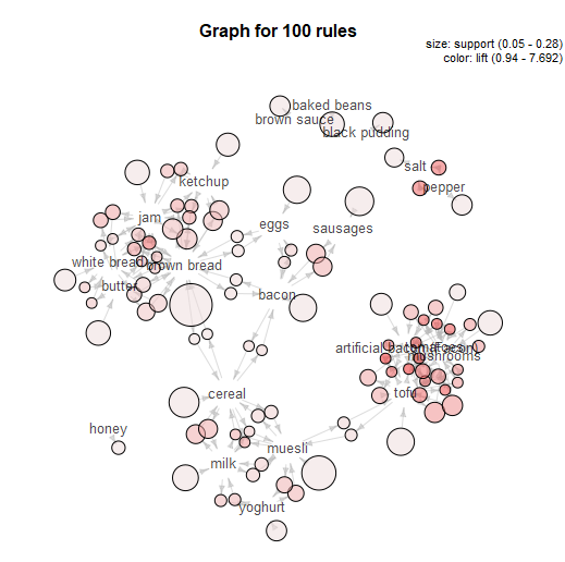
That's basically it for a simple market basket analysis. The MB Inspect tool does also generate some graphics, which I don't normally use that much, although I do like the network graph it makes:

That's the main way of doing market basket analysis in Alteryx, and it's what I do most of the time. But there are several other options, so let's explore what they do as well.
Apriori Association hyperedgesets
In the same Apriori section, there's an option to look at Association hyperedgesets:
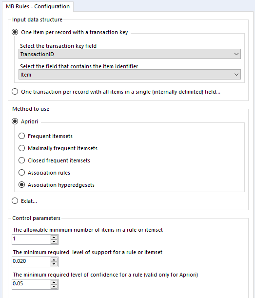
What this does is basically to average across both sides of an association rule. It gives you the same support, the same number of associations, and the average confidence for both sides.
You can see that in the output below.
To explain, let's take the mushrooms/tofu relationship again. This time, it doesn't list an association rule - all you can see is the two items together in one set, ordered alphabetically, like {mushrooms, tofu}.
You can see that the support here (0.12) is the same as the support for both association rules (0.12). However, look at the confidence. And when I say 'confidence', I mean the field called NA.
(Rather unhelpfully, the output of the hyperedgesets option has the column NA and the column NA2. The column NA2 should actually be called NA, as it shows the number of associations, and the column NA should actually be called confidence.)
Anyway, let's look at the confidence (column NA). The figure 0.752941 is the average of the confidence for mushrooms → tofu (0.8) and the confidence for tofu → mushrooms (0.705882).
The minimum confidence setting here applies only to the average confidence, not the individual rules. So for example, if I had set the minimum confidence in the MB Rules tool to 0.73, I would still get the hyperedgeset {mushrooms, tofu} because the average confidence is above 0.73, even though the confidence of the association rule tofu → mushrooms is below 0.73.
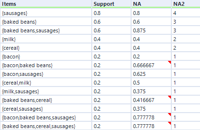
If I go back to the earlier five-transaction dataset, the hyperedgeset average confidence for sausages and baked beans is 0.875. This is the average of the confidence for sausages given baked beans (which is 1) and the confidence for baked beans given sausages (which is 0.75). I think that you can interpret this to mean that if you buy one if the items in that set, there's an 87.5% chance you'll buy one of the other items in that set (or to put it another way, 87.5% of items in this set occurred in combination in a transaction with the other items in this set), but don't quote me on that!
In any case, here's the hyperedgeset results for the five-transaction dataset:
THEORY - PART TWO
Thought we were done with theory? Surprise! Here's a nice little bonus bit, because to cover the other options, we'll need to talk about sets and supersets.
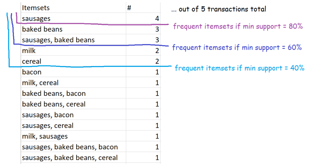
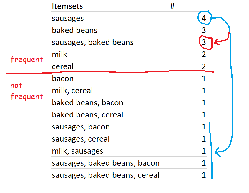
Let's go back to the five-transaction dataset. Here is a list of every single item and combination of items that occur, along with the number of times they occur. At the top, you can see that sausages are bought in four transactions - this doesn't mean that there were four transactions where people only bought sausages, this just means that there were four transactions (of a potentially unlimited size) which contained sausages. At the bottom, you can see that there was one transaction which contained sausages, baked beans, and bacon.
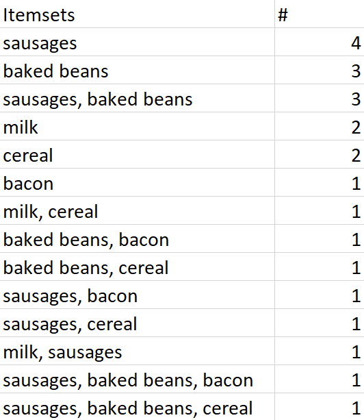
All of these are sets. The set {sausages} is a set made up of a single item - sausages. {sausages, baked beans} is a set made up of two items. And so on. Because they're sets, they get curly brackets around them, like {}, when we're specifically talking about the items as a set rather than a group of items.
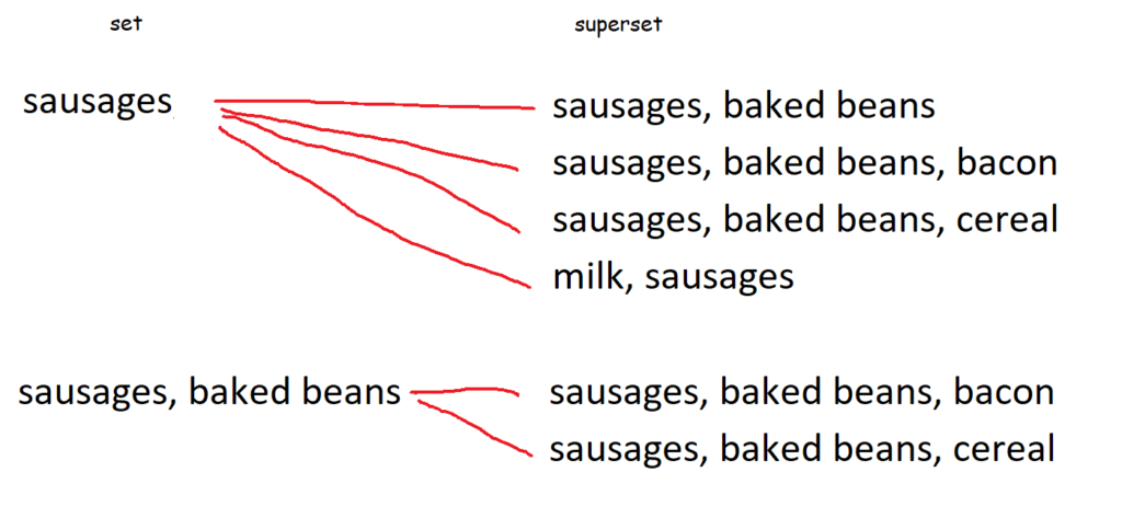
A superset is a set that contains another set. For example, the set {sausages, baked beans} is a superset of the set {sausages}, because the superset fully contains the set. Similarly, the set {sausages, baked beans, bacon} is a superset of the sets {sausages} and {sausages, baked beans}, because the superset fully contains those sets.
This diagram shows every single superset of {sausages} and {sausages, baked beans}:
This is relevant for the next set of options because we'll need to talk about supersets to be able to define frequent itemsets, closed frequent itemsets, and maximally frequent itemsets.
Frequent itemsets
This one is nice and straightforward - it's simply sets of items which occur above your defined level of support. So, for example, if you set 60% as your minimum level of support, then the definition of frequent itemsets is all sets of items which occur in 60% or more of transactions. In our case, that's {sausages}, {baked beans}, and {sausages, baked beans}.
In our five-transaction example, here are some possible frequent itemsets:
Setting the frequency yourself might make it feel like a bit of a circular analysis - 'I want to know what's frequent, so here's my definition of frequent' - but it's pretty useful all the same, because every organisation's data is different. What counts as frequent in a specialist shop might be way higher than a giant supermarket, so this allows you to tailor your analysis differently.
Closed frequent itemsets
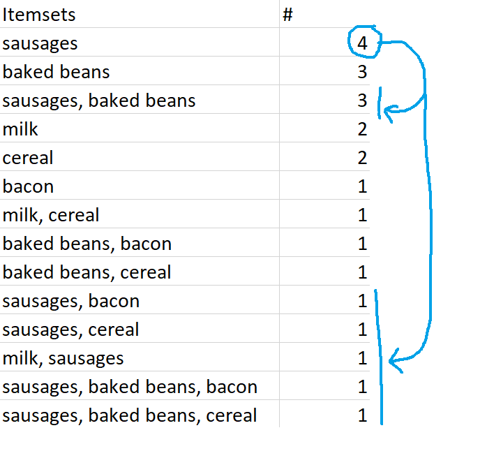
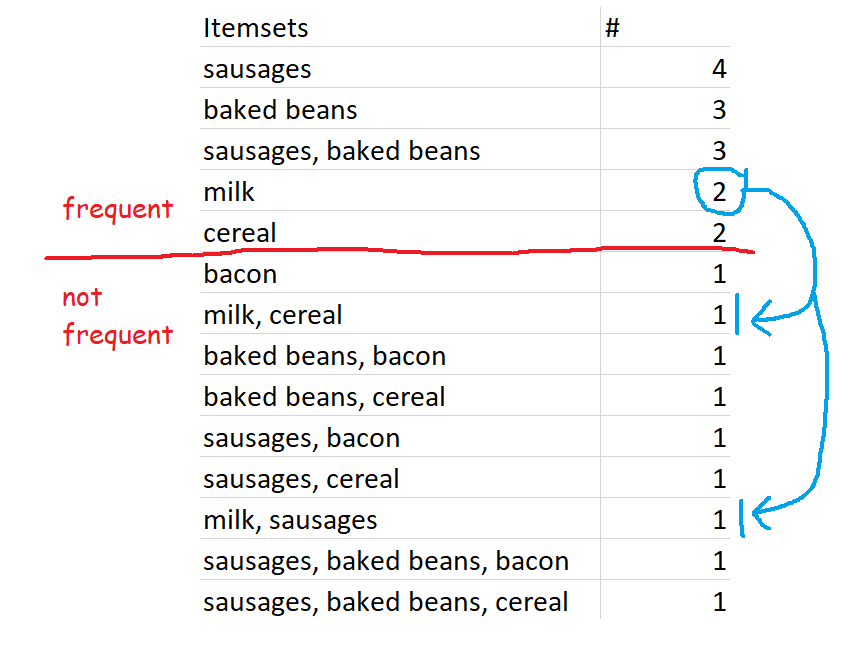
Closed frequent itemsets are sets which are frequent and also occur more frequently than their supersets. For example, let's define frequent as having a minimum support of 0.4 or 40%, which in this dataset works out to occurring in 2 or more transactions. Sausages are in four transactions, so the set {sausages} is a frequent itemset. This is also more frequent than any of the supersets of {sausages}, like {sausages, baked beans} or {sausages, bacon}, so {sausages} is a closed frequent itemset.
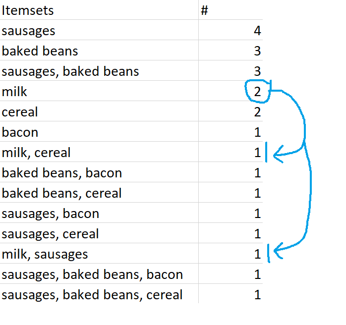
Similarly, {milk} is a closed frequent itemset because it occurs twice - that's frequent according to our 40% definition, and that's more frequent than its supersets, {milk, cereal} and {milk, sausages}.
However, if we increased the minimum support to 0.6, or 60%, then {milk} would no longer be a closed frequent itemset - even though it still fulfils the closed set requirements by being more frequent than its superset, it's no longer frequent by our definition.
Maximally frequent itemsets
Finally, maximally frequent itemsets are frequent itemsets which are more frequent than their supersets, and which do not have any frequent supersets. To put it another way, maximally frequent itemsets are closed frequent itemsets which have no frequent supersets.
{milk} is a closed frequent itemset, and it's also a maximally frequent itemset. This is because {milk} is frequent, {milk} is more frequent than its supersets {milk, cereal} and {milk, sausages}, and its supersets {milk, cereal} and {milk, sausages} are not frequent sets.
However, while {sausages} is both a frequent itemset and a closed frequent itemset, {sausages} is not a maximally frequent itemset. This is because one of {sausages}'s supersets, {sausages, baked beans}, is also a frequent itemset.
...but again, this is because of our preset definition of frequent. If we changed the minimum support for frequent itemsets to 70% rather than 60%, then the set {sausages, baked beans} would no longer be frequent, so {sausages} would be a maximally frequent itemset.
ALTERYX EXAMPLES
Now that we've seen the theory, it's really quick to run these analyses in Alteryx.
You may have noticed that there are two different ways of running a frequent itemsets analysis - one under the apriori method, and one under the eclat method. The only difference is the search algorithm used. The two methods return exactly the same results (well, almost - the order of items with the same NA and Support is slightly different, but that doesn't actually matter, and the results don't join up perfectly, but that's because of joining on a double, so they do join up perfectly if you convert the NA columns to Int16 or something). From what I can tell/from what I've googled, the difference in the search algorithms is that apriori scans through the data multiple times, which makes eclat slightly faster for larger datasets. In my dataset of 100 transactions, it made absolutely no difference to the speed.
So, we can set up the eclat frequent itemsets analysis up like this:
...and here's what the output looks like:
Eagle-eyed readers may have noticed that the output of the eclat frequent itemsets analysis is the same as the apriori hyperedgesets analysis, but without the average confidence column. And it is, but it does run a little quicker.
Onto closed frequent itemsets - if we set up the tool like this:
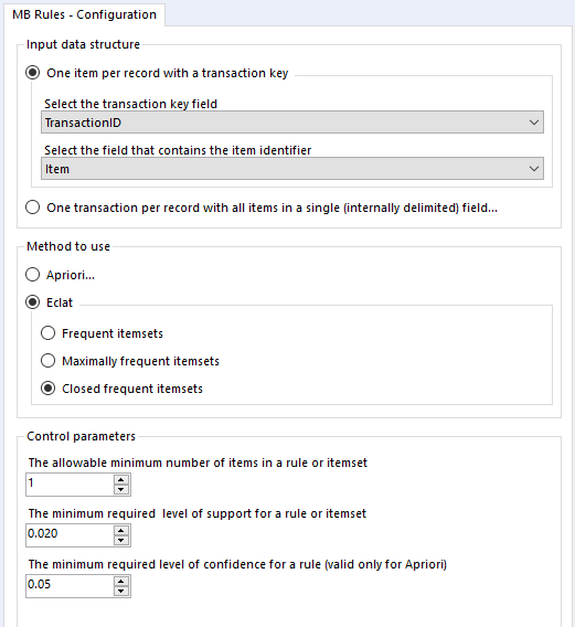
...we get results like this:
At first, this looks identical to the output of the frequent itemsets analysis, but that's only because I'm screenshotting the first few rows. There are less than half the number of itemsets returned by the closed frequent itemsets option.
Finally, let's look at maximal closed frequent itemsets. Again, we'll set it up like this:
...and again, here's the output:
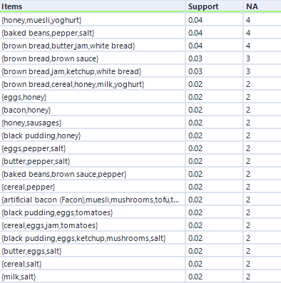
This output structure is identical to the other two, but the results are more noticeably different. The honey/muesli/yoghurt combo is the most frequent maximally frequent itemset.
Application
I've written about applying market basket analysis to your data before, and this has turned into a really long blog post, so I won't cover it in full here. But, as a shop keeper, I'd use the results of this analysis in Gwilym's Breakfast Goods Co. to explore what to put on sale together, what not to put on sale together, and so on. For example, mushrooms and tofu are the combination with the highest lift, so if I'd accidentally overstocked on tofu and needed to sell it off quickly, I'd put it on special offer with mushrooms and put it in the vegetable (or fungus-pretending-to-be-a-vegetable) aisle. But if I'd done my supply chain planning well, I could use the strong association between mushrooms and tofu to get people to buy other things. For example, people who buy tofu also buy artificial bacon (Facon), so I could use people's tendency to buy tofu and mushrooms together by putting them in the same aisle but sandwiching artificial bacon (Facon) between the two. This would mean that people looking for the tried and trusted mushroom/tofu combination are going to be looking at artificial bacon (Facon) at the same time, and hopefully they'll pick it up and try it out.